Chapter 7 Differential OCR analysis
Differential peak analysis can help us identify differences in gene regulation under different conditions and reveal important regulatory mechanisms in cellular states and biological processes. This section of the analysis is an important step in the search for differential TFBSs and is the basis for performing a functional difference analysis.
7.1 Using DEseq2 to identify differentail OCR (Two groups)
DESeq2 is an R package for differential expression analysis, but can also be used for differential peak analysis with ATAC-seq. Here we use DEseq2 as an example to identify the difference peaks between the two groups.
data(Diff_Analysis_Example)
quant_data <- Diff_Analysis_Example
diff_res <- getDiffPeak(norm_data = quant_data, condition = c("Control","Exper"), control = "Control", experment = "Exper",rep_N= 2)
## converting counts to integer mode## estimating size factors## estimating dispersions## gene-wise dispersion estimates: 22 workers## mean-dispersion relationship## final dispersion estimates, fitting model and testing: 22 workershead(diff_res)## baseMean log2FoldChange lfcSE stat pvalue
## chr1:10016-10607 54.030792 0.5635555 0.5826459 0.9672349 0.3334266
## chr1:237589-237928 11.903993 0.3358489 0.7164559 0.4687643 0.6392381
## chr1:521379-521712 6.946804 0.1798363 0.8110918 0.2217212 0.8245309
## chr1:540496-541113 8.700218 -0.1107456 0.7780795 -0.1423320 0.8868178
## chr1:559303-559603 8.693440 -0.2740060 0.7751323 -0.3534957 0.7237168
## chr1:564421-565042 24.555285 0.2952452 0.6325501 0.4667538 0.6406760
## padj sig
## chr1:10016-10607 0.7779954 None
## chr1:237589-237928 0.9452912 None
## chr1:521379-521712 0.9800009 None
## chr1:540496-541113 0.9845317 None
## chr1:559303-559603 0.9657660 None
## chr1:564421-565042 0.9456528 NoneWe can use the commonly used volcano diagram to show these differential peaks.
plotVolcano(diff_data = diff_res)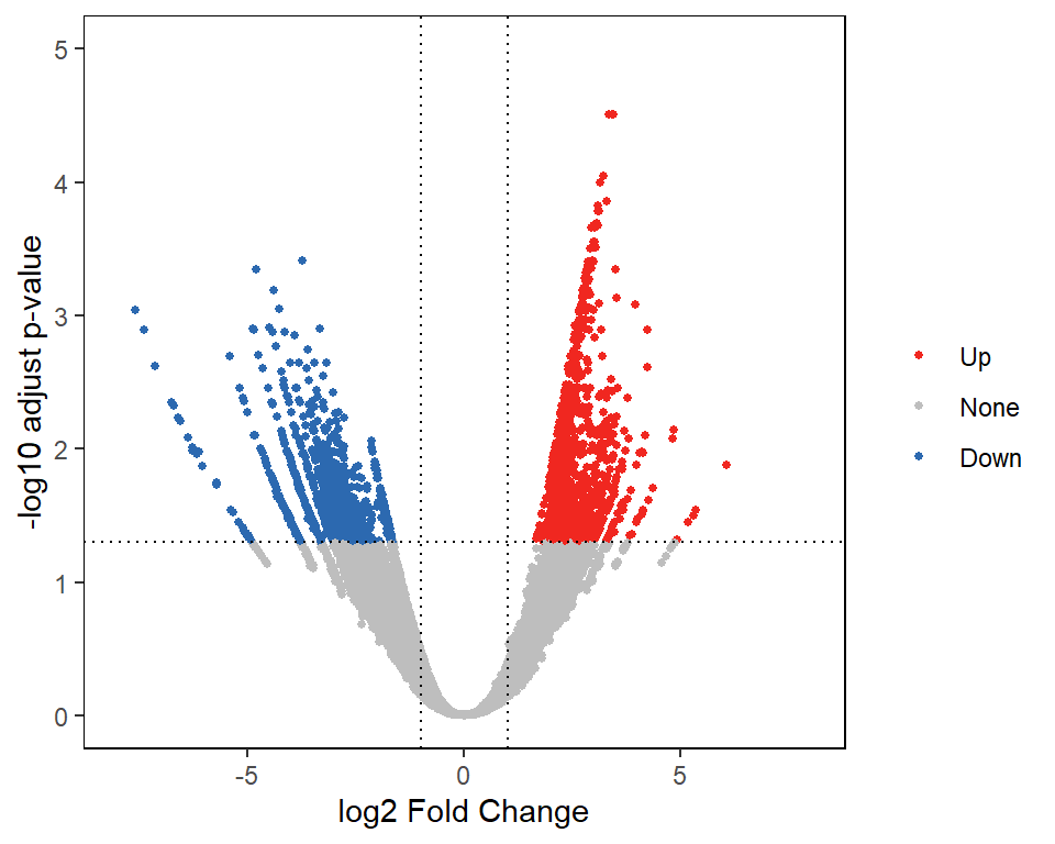
7.2 Get the differential peaks target genes
Having obtained these differential peaks, we were more interested in knowing which genes’ expression might be affected by these differential peaks. In general, we annotate these differential peaks to the nearest genes. We can run the getDiffTargetGenes function to complete this analysis.
target <- getDiffTargetGenes(diff_data=diff_res)
head(target)
## chrom start end baseMean log2FoldChange lfcSE stat
## 1 chr1 100009953 100010254 20.142897 -0.4939808 0.6575732 -0.7512181
## 2 chr1 100012048 100012826 23.103692 -0.3060881 0.6464743 -0.4734730
## 3 chr1 100017890 100018149 8.223809 -0.8358235 0.8052071 -1.0380231
## 4 chr1 100023076 100023997 22.811175 0.2890909 0.6505642 0.4443696
## 5 chr1 10002486 10002743 8.659492 1.0989500 0.7945523 1.3831059
## 6 chr1 10002897 10003700 55.147809 -0.1827790 0.5806837 -0.3147652
## pvalue padj sig peak_center TSS gene strand distance
## 1 0.4525214 0.8669849 None 100010103 99929934 1 + -80169
## 2 0.6358758 0.9436658 None 100012437 99929934 1 + -82503
## 3 0.2992593 0.7424509 None 100018019 99929934 1 + -88085
## 4 0.6567754 0.9507410 None 100023536 100111499 1 + 87963
## 5 0.1666324 0.5544505 None 10002614 10003465 1 - -851
## 6 0.7529400 0.9699603 None 10003298 10003465 1 - -1677.3 PlotMA
In addition, we can also use the plotMA function to display information about both the difference peaks and their summit to the nearest TSS distance.
plotMA(target)## Warning: Removed 21 rows containing missing values (`geom_point()`).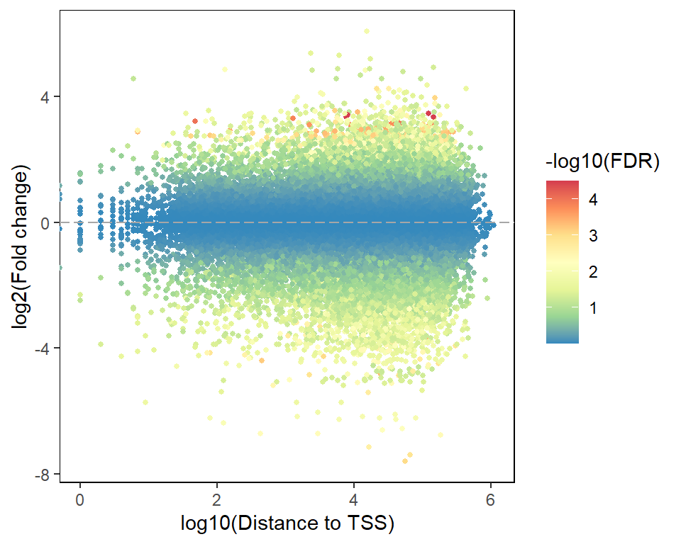
7.4 Compare the three samples chromatin accessibility (Three samples)
For the analysis of differences among the three groups, a common method is a two-by-two comparison. Here, we are inspired by R. H. Ramírez-González et al. For three groups of ATAC-seq data, we can use this triads approach to get the difference peaks at the same time and visualized with a ternary plot. We take the previous quantized matrix and extract the Bulk_B, Mem_B, Naive_B to compare the differences between the three groups.
data("All_quant_data")
quant_data <- All_quant_data[,1:3]
getTriads(group_name=c("Bulk_B","Mem_B","Naive_B"), quant_df = quant_data, return_matrix=F)
## Registered S3 methods overwritten by 'ggtern':
## method from
## grid.draw.ggplot ggplot2
## plot.ggplot ggplot2
## print.ggplot ggplot2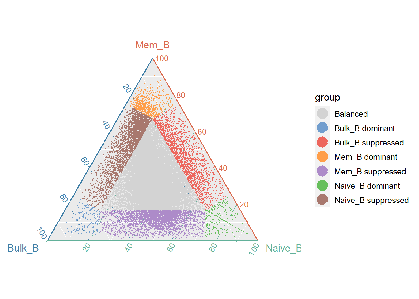 We can categorize them into seven categories and use a boxplot to show if their categorization is accurate.
triads_res <- getTriads(group_name=c("Bulk_B","Mem_B","Naive_B"), quant_df = quant_data, return_matrix=T)
plotTriads(triads_data = triads_res)
## Using group as id variables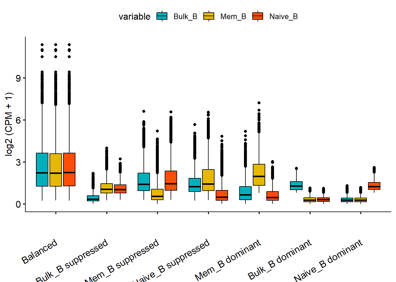
Finally, we can similarly use the getTraidsTargetGenes function to get the target genes for each category of peaks.
triads_targets <- getTriadsTargetGenes(triads_data = triads_res)
head(triads_targets)
## chrom Peak_center Bulk_B Mem_B Naive_B group Peak_start
## 1 chr1 10002672 10.9749479 8.274032 10.8202002 Balanced 10002429
## 2 chr1 10003391 49.4307820 41.862457 46.2388672 Balanced 10002983
## 3 chr1 10010875 25.6538466 23.160242 25.3581749 Balanced 10010299
## 4 chr1 100151436 2.8350983 3.277752 1.8329218 Balanced 100151228
## 5 chr1 100165806 0.6880433 0.615438 0.4909362 Balanced 100165637
## 6 chr1 100194636 0.8866477 1.970254 1.2235983 Balanced 100194551
## Peak_end TSS gene strand distance
## 1 10002916 10003465 ENSG00000162441 - -793
## 2 10003799 10003465 ENSG00000162441 - -74
## 3 10011452 10003465 ENSG00000162441 - 7410
## 4 100151645 100163798 ENSG00000223656 + 12362
## 5 100165976 100163798 ENSG00000223656 + -2008
## 6 100194721 100163798 ENSG00000223656 + -30838