Chapter 9 Time Course Data
Biological time course data are a common experimental design in research and are important for understanding the dynamic processes of biological systems, revealing regulatory mechanisms, predicting trends, and individual differences and responses.
Time-course ATAC-seq can help us decipher the following aspects:
Dynamic chromatin accessibility: Time-course ATAC-seq enables the investigation of dynamic changes in chromatin accessibility over time. It allows us to identify genomic regions that undergo opening or closing during specific time points, shedding light on the temporal regulation of chromatin structure.
Transcriptional regulation: By comparing ATAC-seq profiles across multiple time points, we can unravel the regulatory elements and transcription factor binding sites associated with specific temporal patterns of chromatin accessibility. This information provides insights into the dynamic regulation of gene expression during different stages or conditions.
Cell fate determination: Time-course ATAC-seq data facilitates the exploration of chromatin dynamics during cellular differentiation and development. It helps uncover the changes in chromatin accessibility associated with cell fate decisions and provides a molecular understanding of the underlying mechanisms governing cell fate determination.
Temporal gene regulatory networks: Integrating time-course ATAC-seq data with gene expression data allows the construction of temporal gene regulatory networks. These networks provide a comprehensive view of the regulatory interactions and signaling pathways involved in orchestrating gene expression changes over time.
Disease progression and response: Time-course ATAC-seq analysis can elucidate the dynamic alterations in chromatin accessibility associated with disease progression, treatment response, or cellular response to external stimuli. It aids in identifying key regulatory elements and pathways implicated in disease development and therapeutic interventions.
In summary, time-course ATAC-seq data provides a powerful tool to decipher the dynamic nature of chromatin accessibility and its impact on gene regulation, cell fate determination, and disease processes. By capturing temporal changes in chromatin accessibility, we gain valuable insights into the underlying molecular mechanisms driving biological processes and disease progression.
When analyzing changes over time in ATAC-seq data, our primary focus is on identifying the OCRs that undergo changes throughout the process. Therefore, our input should consist of the differential OCRs between each pair of time points. Unlike the pseudotime for single cells, our bulk ATAC-seq data is generated at predetermined time points, eliminating the need to infer the temporal order between samples.
9.1 Fitting time with ATAC-seq
Thus for normalized quantitative data, we first use getSpecificPeak or getTopSpecifcPeaks to get dynamic difference OCRs.
dynamic_ocrs <- getTopSpecifcPeaks(spm_data = spm, norm_data = quant_data, top_N = 1000, save_path = "F:/cisDynet/example/", file_prefix = "Top1000_raw_data")We then use getTimeATAC to fit these dynamic OCRs in order of time points.
getTimeATAC(norm_data = dynamic_ocrs)## `use_raster` is automatically set to TRUE for a matrix with more than
## 2000 rows. You can control `use_raster` argument by explicitly setting
## TRUE/FALSE to it.
##
## Set `ht_opt$message = FALSE` to turn off this message.## 'magick' package is suggested to install to give better rasterization.
##
## Set `ht_opt$message = FALSE` to turn off this message.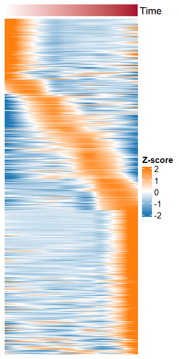
9.2 Integration with RNA-seq
Of course we can also use the information from peak2gene to get the current dynamic OCR corresponding to the expression change of the target gene.
peak_time <- getTimeATAC(norm_data = dynamic_ocrs, return_matrix = T)
getTimeRNA(peak_time = peak_time, peak2gene = "F:/cisDynet/example/Peak2Gene_All_Links.rds",
           rna_matrix = "F:/cisDynet/example/RNA_TPM_Norm_Data.tsv",corr_cutoff = 0.4)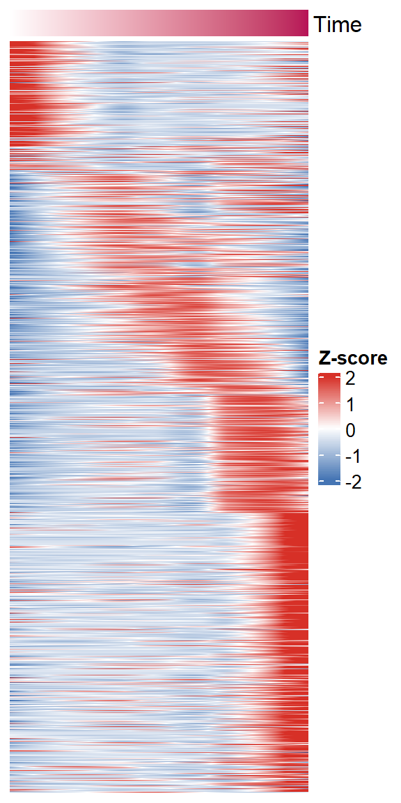
9.3 Get fitting time genes
We can use getTimeGene to extract a list of dynamically changing genes.
gene <- getTimeGene(peak_time = peak_time, peak2gene = "F:/cisDynet/example/Peak2Gene_All_Links.rds",
                    rna_matrix = "F:/cisDynet/example/RNA_TPM_Norm_Data.tsv",corr_cutoff = 0.4)
head(gene)
## Gene Peak
## 1 ENSG00000229106 chr1:24239631-24240158
## 2 ENSG00000142583 chr1:9129431-9130125
## 3 ENSG00000128815 chr10:49891876-49892358
## 4 ENSG00000213057 chr1:178548735-178549177
## 5 ENSG00000213057 chr1:178544701-178545421
## 6 ENSG00000132906 chr1:15898208-158988229.4 Integration with ATAC / RNA-seq
We label the right side of the heatmap based on the genes obtained above. You need to prepare a file in this format.
##              gene    name
## 1 ENSG00000085831  TTC39A
## 2 ENSG00000150316   CWC15
## 3 ENSG00000169504   CLIC4
## 4 ENSG00000161955 TNFSF13
## 5 ENSG00000095585    BLNK
## 6 ENSG00000169607  CKAP2L
Next we can use the plotTimeAll function to draw the heatmap of ATAC and RNA at the same time and label some genes.
plotTimeAll(norm_data = dynamic_ocrs,
            peak2gene = "F:/cisDynet/example/Peak2Gene_All_Links.rds",
            rna_matrix = "F:/cisDynet/example/RNA_TPM_Norm_Data.tsv",
            label = "F:/cisDynet/example/time_anno.txt")
## 2023-10-23 14:51:43 Calculating ATAC time...## 2023-10-23 14:51:57 Calculating RNA time...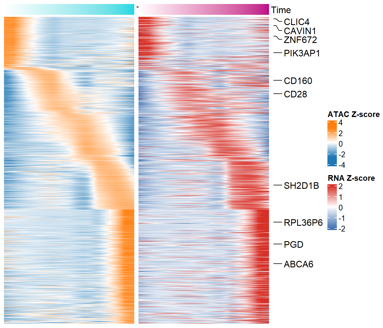
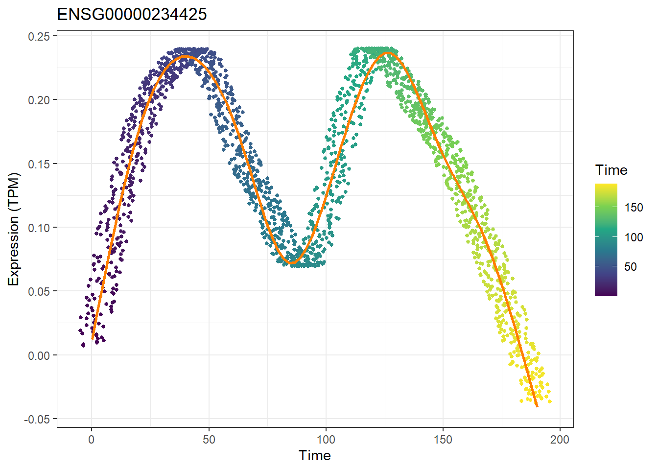
We can also use plotTimeGene to draw dynamic changes in the expression of individual genes.
plotTimeGene(peak_time = peak_time,peak2gene = "F:/cisDynet/example/Peak2Gene_All_Links.rds",
             rna_matrix = "F:/cisDynet/example/RNA_TPM_Norm_Data.tsv",corr_cutoff = 0.4,gene = "ENSG00000234425")
## `geom_smooth()` using method = 'gam' and formula = 'y ~ s(x, bs = "cs")'